Section author: Stephanie Juneau <stephanie.juneau@noirlab.edu>
1.2.1. Star/galaxy/QSO classification
This science case starts from an imaging survey and takes steps toward classifying objects that are detected into stars, galaxies and quasi-stellar-objects (QSOs).
The Jypter notebook file and a rendered HTML version are available on GitHub:
You will also find them on your Data Lab notebook server, in the notebooks-latest/
folder. [It’s best to first fetch the newest notebooks].
1.2.1.1. Background
Imaging surveys encompass a number of different astronomical objects, generally including stars, galaxies and QSOs. Each category of objects is interesting in their own right, but not necessarily straightforward to classify. In particular, near the spatial resolution limit, compact galaxies, QSOs and stars may all appear as point sources.
In order to differentiate between these types of objects, work has been done extracting information from images such as photometry (magnitudes and colors) and/or the shape of light profiles. When available, spectroscopy can contribute more information thanks to spectral features (continuum shape, emission lines, absorption lines, etc.) and redshift information.
Here, we focus on the case where only imaging (photometry) is available.
1.2.1.2. Goal
We will investigate colors and model shapes (type) of astronomical objects in the DESI imaging Legacy Survey in order to classify them into stars, galaxies, and QSOs.
1.2.1.3. Data
We use g,r,z photometry, WISE photometry, and object type from the LS DR9 Tractor catalog. Optical and infrared photometry is combined to plot bivariate distributions in color-color space.
WISE photometry is restricted to the more sensitive observations from the first two channels W1 and W2, respectively centered on 3.4 and 4.6 microns.
The object type can be one of these five: PSF, SIMP, EXP, DEV, SER, as defined in the documentation.
Lastly, we retrieve postage stamp images from the LS team Sky Viewer using a set of URL’s and downloading/caching images.
1.2.1.4. Technique
The technique is to query the LS Tractor catalog for photometric information including magnitudes which were corrected for foreground extinction by using the Milky Way transmission values, and the object model type (to have information on the shape of the light profile).
This information is then combined to separate population of points corresponding to object classes. Using color cuts for target selection or photometric identification is a common approach. We note that alternative approaches include using Machine Learning (e.g., Random Forest) in order to classify source types based on a training set of pre-classified objects.
1.2.1.5. Data Lab Workflow
The first steps are to import libraries that will be needed, and to authenticate.
Then, we query relevant columns from the tractor table of the LS DR9 database. In this case, we query deredenned magnitudes g, r, z, W1, and W2 as well as the object type, and the RA and dec coordinates. We require a signal-to-noise ratio greater than 5 in each of the g, r, z, W1, and W2 bands.
query = """SELECT dered_mag_g as gmag, dered_mag_r as rmag,
            dered_mag_z as zmag, dered_mag_w1 as w1mag, dered_mag_w2 as w2mag, type,
            snr_g, snr_r, snr_z, ra, dec
         FROM ls_dr9.tractor
         WHERE (snr_g>5 and snr_r>5 and snr_z>5 and snr_w1>5 and snr_w2>5)
         LIMIT 400000"""
From the query results, we can plot color-color diagrams with any combination of colors. We select to combine optical and infrared colors, and look at both the population of objects overall, and split by object type. The RA and Dec coordinates will be used to retrieve a few image cutouts.
One could potentially extend this work by computing additional colors or using more information such as the magnitudes or goodness-of-fit of the model (chi squared values).
1.2.1.6. Output

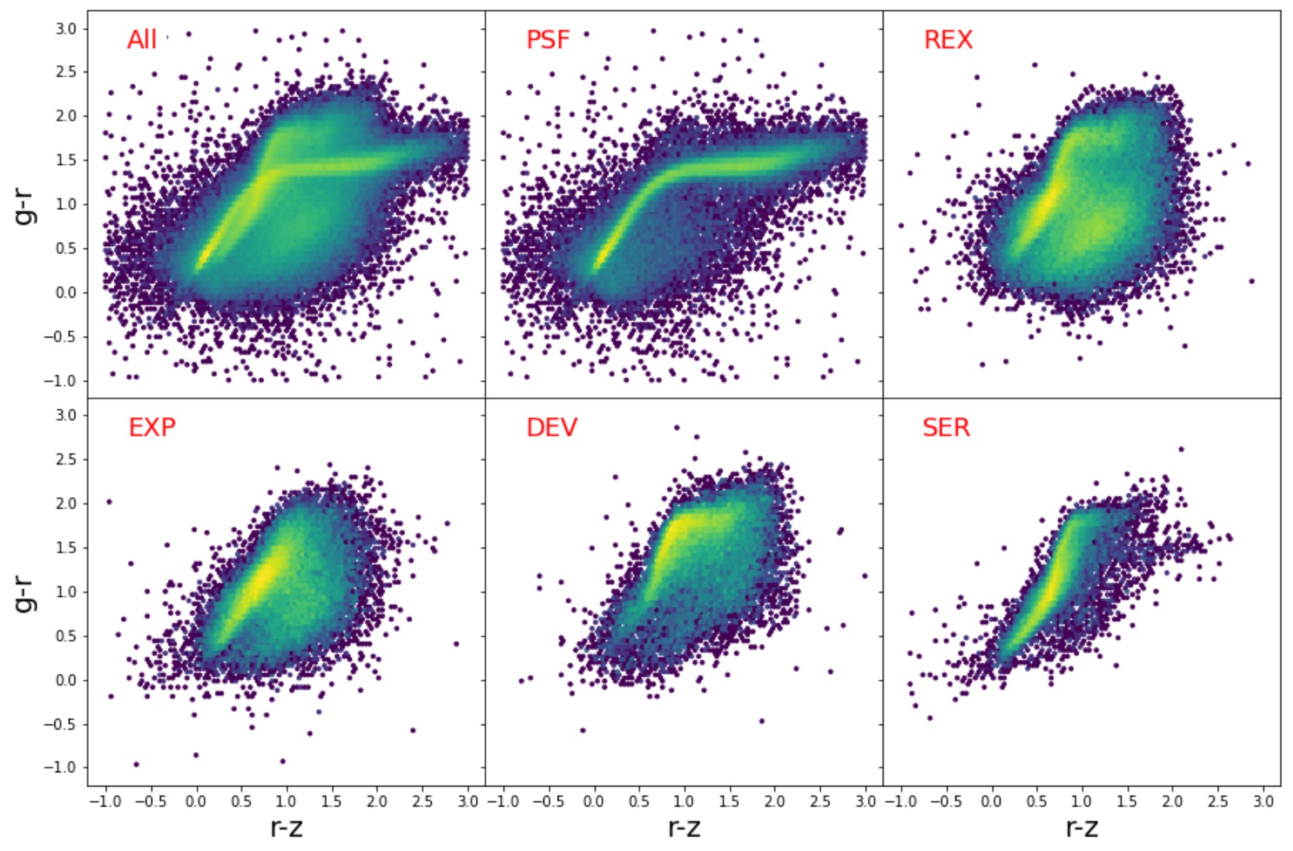
Figure: Color-color diagram using LS g-r and r-z colors. The top left panel shows all objects from the query. The remaining five panels are split per Type as labeled.
The figure above shows structures in the bivariate distributions. In the top left panel, labeled ‘All’, we can see two branches that cross over each other, as well as a cloud of points below the branches. The remaining panels indicate that one of the branches corresponds to the stellar locus (PSF), while the other branch is a blend of galaxies with types REX, EXP, DEV & SER. The cloud of points is a mixture of PSF, REX & EXP, perhaps including QSOs and compact galaxies. More work would be needed to confirm these classifications.
