Section author: Alice Jacques <alice.jacques@noirlab.edu>, Knut Olsen <knut.olsen@noirlab.edu>, Robert Nikutta <robert.nikutta@noirlab.edu>
Version: 20250924
1.5.2. Simple Image Access (SIA)
The Simple Image Access (SIA) service provides capabilities for the discovery, description, access, and retrieval of multi-dimensional image datasets, including 2-D images as well as datacubes of three or more dimensions. Use of the SIA service requires the external PyVO package, and the URL of the SIA service endpoint that you will use. Data Lab has a general SIA service containing all available images from NOIRLab Science Archive (NSA), as well as a number of survey-specific services.
The SIA service tool works to identify the set of images in an image collection that overlap the position at which an image cutout is desired. It returns a table of potential images containing information (metadata) typically found in the image headers (filter, exposure time, time of observation, etc.) as well as a URL pointing to the image cutout itself. Getting image cutouts is thus a three-step process:
choose an image collection
call the SIA service for that collection to retrieve information about images that overlap a position of interest
retrieve the image cutouts by accessing the URLs for the selected images in the table of information
1.5.2.1. Choosing an image collection
Choosing a specific image collection is done by selecting the URL that points to that collection. Here we list the SIA service endpoints for different image collections:
Name |
Description |
DEF_ACCESS_URL |
|---|---|---|
calibrated_all |
All Instrument calibrated images |
|
calibrated/des_y1 |
DES Year-1 calibrated images |
|
calibrated/des_y2 |
DES Year-2 calibrated images |
|
calibrated/des_y3 |
DES Year-3 calibrated images |
|
calibrated/des_y4 |
DES Year-4 calibrated images |
|
calibrated/nsa |
NSA calibrated images |
|
calibrated/smash_dr1 |
SMASH DR1 calibrated images |
|
calibrated/smash_dr2 |
SMASH DR2 calibrated images |
|
coadd_all |
All coadded images |
|
coadd/decaps_dr1 |
DECaPS DR1 coadd images |
|
coadd/des_dr1 |
DES DR1 coadd images |
|
coadd/des_sva |
DES SVA coadd images |
|
coadd/ls_dr8 |
DECaLS DR8 coadd images |
|
coadd/ls_dr9 |
DECaLS DR9 coadd images |
|
coadd/nsa |
NSA coadd images |
|
coadd/smash_dr1 |
SMASH DR1 coadd images |
|
coadd/smash_dr2 |
SMASH DR2 coadd images |
|
decaps_dr1 |
DECaPS DR1 images |
|
decaps_dr2 |
DECaPS DR2 images |
|
delve_dr3 |
DELVE DR3 images |
|
demcels_dr1 |
DeMCELS DR1 images |
|
des_dr1 |
DES DR1 images |
|
des_dr2 |
DES DR2 images |
|
des_dr2_se |
DES DR2 single-epoch images |
|
des_sva1 |
DES SVA1 images |
|
des_y1 |
DES Year-1 images |
|
des_y2 |
DES Year-2 images |
|
des_y3 |
DES Year-3 images |
|
des_y4 |
DES Year-4 images |
|
gogreen_dr1 |
GOGREEN DR1 images |
|
gogreen_dr2 |
GOGREEN DR2 images |
|
ls_dr8 |
DECaLS DR8 images |
|
ls_dr9 |
DECaLS DR9 images |
|
ls_dr10 |
DECaLS DR10 images |
|
nsa |
NOIRLab Science Archive |
|
nsc_dr2 |
NOIRLab Source Catalog DR2 |
|
raw/nsa |
NSA Raw images |
|
raw_all |
All Raw images |
|
raw/smash_dr1 |
SMASH DR1 raw images |
|
raw/smash_dr2 |
SMASH DR2 raw images |
|
sdss_dr9 |
SDSS DR9 sky-subtracted images |
|
smash_dr1 |
SMASH DR1 images |
|
smash_dr2 |
SMASH DR2 images |
|
splus_dr1 |
S-PLUS DR1 images |
|
splus_edr |
S-PLUS EDR images |
|
stripe82/calibrated |
Calibrated images in Stripe82 |
|
stripe82/coadd |
Coadd images in Stripe82 |
|
stripe82/decaps_dr1 |
DECAPS DR1 images in Stripe82 |
|
stripe82/des_dr1 |
DES DR1 images in Stripe82 |
|
stripe82/des_dr2 |
DES DR2 images in Stripe82 |
|
stripe82/des_sva1 |
DES SVA1 images in Stripe82 |
|
stripe82/des_y1 |
DES Year-1 images in Stripe82 |
|
stripe82/des_y2 |
DES Year-2 images in Stripe82 |
|
stripe82/des_y3 |
DES Year-3 images in Stripe82 |
|
stripe82/des_y4 |
DES Year-4 images in Stripe82 |
|
stripe82/ls_dr8 |
DECaLS DR8 images in Stripe82 |
|
stripe82/ls_dr9 |
DECaLS DR9 images in Stripe82 |
|
stripe82/nsa |
NOIRLab Science Archive images in Stripe82 |
|
stripe82/nsc_dr2 |
NSC DR2 images in Stripe82 |
|
stripe82/raw |
Raw images in Stripe82 |
|
stripe82/sdss_dr9 |
SDSS DR9 images in Stripe82 |
|
stripe82/smash_dr1 |
SMASH DR1 images in Stripe82 |
|
stripe82/smash_dr2 |
SMASH DR2 images in Stripe82 |
|
stripe82/splus_dr1 |
S-PLUS DR1 images in Stripe82 |
|
stripe82/splus_edr |
S-PLUS EDR images in Stripe82 |
|
1.5.2.2. Retrieving image information
We can use the search method of the SIA service object to perform a search within a specified field of view (fov) size. The search method takes the following as arguments:
(ra,dec) - a tuple containing the RA and Dec of the object in decimal degrees
fov - a tuple with the size of the cutout in each direction in degrees
For example, we will pick a location in SDSS Stripe 82 in the subset of images from the NOIRLab Science Archive (nsa) that overlap with SDSS Stripe 82:
> DEF_ACCESS_URL = "https://datalab.noirlab.edu/sia/stripe82/nsa"
> svc_stripe82 = sia.SIAService(DEF_ACCESS_URL)
We use the SDSS Stripe 82-specific SIA service above to retrieve the image information for an image cutout whose fov size is 6x6 arcmin (0.1x0.1 degrees). We want the result to be an Astropy table, so we add .to_table() at the end of the call:
> ra = 335.0
> dec = 0.0
> fov = 0.1
> imgTable = svc_stripe82.search((ra,dec), (fov/np.cos(dec*np.pi/180), fov), verbosity=2).to_table()
NOTE the search method works in RA and Dec in degrees, and does not account for the convergence of lines of RA toward the poles, so we divide by a cos(dec) term in the RA fov argument.
The result is a table of metadata for images that overlap the search position.
1.5.2.3. Retrieving image cutouts
In the result table of metadata for images obtained above, the column access_url contains the link to retrieve the image cutout. We can filter the table on any of the columns to narrow down the list to just the cutouts we want. Here we’ll select stacked images (proctype=Stack and prodtype=image) observed in the g filter (obs_bandpass that contains the letter ‘g’):
> sel = (imgTable['proctype'].astype(str)=='Stack') & (imgTable['prodtype'].astype(str)=='image') & (startswith(imgTable['obs_bandpass'].astype(str),'g'))
From the filtered table we will pick a row and retrieve the image:
> row = imgTable[sel][1]
> url = row['access_url'].decode() # get the download URL
> filename = download_file(url,cache=True,show_progress=False,timeout=120)
> hdu = fits.open(filename)[0]
> image = hdu.data
> hdr = hdu.header
> wcs = WCS(hdr) # WCS info from header to convert pixel coords to world coords
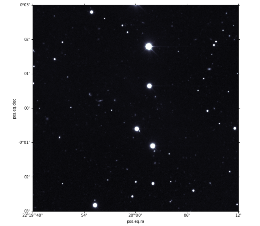
Then we’ll display the image. Note that the image might not be square for a variety of reasons, such as that the image cutout ran into a chip edge along one axis.
> fig = plt.figure(figsize=(10,10))
> ax = fig.add_subplot(projection=wcs)
> ax.imshow(image,origin='lower',cmap='bone',vmin=image.min(),vmax=image.min()+(image.max()-image.min())/170.)

1.5.2.4. Resources and References
See our How To Use SIA Service Jupyter notebook for example usage.
For more background on the SIA protocol, see the IVOA document that describes it.
