Section author: Robert Nikutta <robert.nikutta@noirlab.edu>
1.2.3. Discover faint Milky Way dwarf galaxies
We will explore a way to (almost) automatically discover overdensities in the sky, which can potentially be Milky Way dwarf galaxies.
The Jypter notebook file and a rendered HTML version are available on GitHub:
Dwarf galaxy notebooks with other datasets
You will also find them on your Data Lab notebook server, in the notebooks-latest/
folder. [It’s best to first fetch the newest notebooks].
More on Jupyter notebooks.
Below we explain the motivation, methods, and Data Lab workflow, with snippets of the notebook in key places.
1.2.3.1. Background
Ultrafaint dwarf galaxies are crucial to understanding many aspects of the universe. For instance, they are dominated by dark matter; their localization in space can thus trace the large-scale structure of the dark matter distribution. Furthermore, dwarf galaxies are suspected to host intermediate-mass black holes (IMBH), which so far have eluded efforts to find them. IMBHs will naturally bridge the gap between the solar-mass black hole and super-massive blackholes that reside at the center of virtually every large galaxy.
The techniques described here follow Martin at al. (2015) (1).
1.2.3.2. Goal
We will attempt to automatically identify significant stellar overdensities in one field of the SMASH survey (2), and inspect by eye the images around the peaks found. We will also plot and inspect the color-magnitude diagrams (CMD) of the stars around the identified density peaks.
1.2.3.3. Data
We will query the averaged photometry table from the SMASH survey (2), and specifically focus on field #169 there. We will limit the query to photometry taken only with long exposures (depthflag>1), avoid broad objects (|sharp|<0.5), and pick blue objects (-0.4 < g-r < 0.4), since dwarf galaxies show an excess of old, metal-poor, blue stars.
1.2.3.4. Technique
We will identify stellar overdensities in the field by convolving the 2-d spatial distribution of stars (i.e. a 2-d histogram image) with two Gaussian kernels of different widths. The difference of these two convolutions is akin to a Mexican Hat type wavelet that rejects density signatures outside the range of spatial sizes spanned by the two kernel widths. Similar techniques have been used e.g. for galaxy clusters (3) and other dwarf galaxies (4).
Once density peaks are identified, we will demonstrate how to use the built-in Simple Image Access (SIA) service to retrieve images of the sky at the peak locations.
1.2.3.5. Data Lab Workflow
We will proceed with these steps:
apply a differential Gaussian kernel convolution to bring out overdensities
download & inspect images via Simple Image Access (SIA) protocol
1.2.3.5.1. Data retrieval
We will select stars in from one field (#169) in the SMASH survey based on their blue colors (g-r), while applying some quality cuts. The database and table are smash_dr1.object, and we’ll ask for the ra, dec, gmag, rmag, imag columns.
 1field = 169 # SMASH field number to query
 2
 3# Create the query string; SQL keyword capitalized for clarity
 4#   depth > 1 = no short exposures please
 5#   ndetr, ndetg > 3 = more than 3 detections in r & g bands
 6#   abs(sharp) < 0.5 = avoid broad objects
 7query =\
 8"""SELECT ra,dec,gmag,rmag,imag
 9   FROM smash_dr1.object
10   WHERE fieldid = '{:d}' AND
11         depthflag > 1 AND
12         ndetr > 3 AND ndetg > 3 AND
13         abs(sharp) < 0.5 AND
14         gmag BETWEEN 9 AND 25 AND
15         (gmag-rmag) BETWEEN -0.4 AND 0.4""".format(field)
Submit the query, and convert the returned CSV table to a Pandas dataframe for convenience:
from dl import authClient as ac, queryClient as qc
from dl.helpers.utils import convert
response = qc.query(query) # response is by default a CSV-formatted string
R = convert(response,'pandas') # R is a pandas dataframe
print("Number of objects:", R.shape[0])
print(R.head())
Returning Pandas dataframe
Number of objects: 104973
           ra        dec       gmag       rmag       imag
0  184.876674 -32.873511  24.746605  24.838743  24.185682
1  184.876606 -32.870861  24.156397  24.068817  23.074945
2  184.875853 -32.867214  24.084047  24.028061  23.630045
3  184.877080 -32.869780  24.482061  24.446104  23.858896
4  184.878492 -32.866905  24.678942  24.714973  24.624266
1.2.3.5.2. Differential convolution
Equipped with 100k+ RA and Dec positions, let’s plot a 2-d histogram of their distributions in the sky.
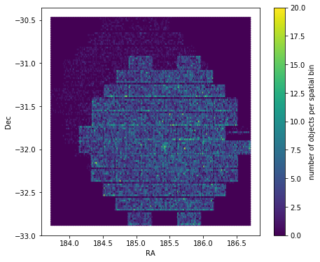
2-d distribution of selected objects in SMASH field 169.
You may be able to see a faint overdensity by eye already, but we want to do better. We can write a function that convolves this image with two Gaussian kernels of different sizes. The Jupyter notebooks in https://github.com/astro-datalab/notebooks-latest/tree/master/03_ScienceExamples/DwarfGalaxies shows the function code.
We compute the convolutions with kernels 2 and 20 arcminutes in size, and plot their difference:
small_k, big_k = 2., 20.  # kernel sizes in arcminutes
raw, extent, delta, clipped, dsigma = dwarf_filter(R['ra'],R['dec'],fwhm_small=small_k,fwhm_big=big_k)
im = plt.imshow(clipped)
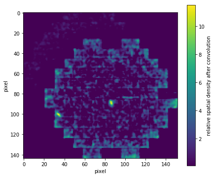
The 2-d spatial histogram, after differential convolution with kernels 2 and 20 arcmin in size.
The enhancements around the edges of the field are due to the convolution being sensitive to discontinuities. But there are a few density peaks very clearly visible inside the field. Let’s investigate them.
1.2.3.5.3. Automatically find peaks
To automate the procedure and free ourselves from subjective judgment, we can identify significant peaks in the convolved 2-d histogram automatically:
from astropy import stats
from photutils import find_peaks
mean, median, std = stats.sigma_clipped_stats(clipped,sigma=3.0,iters=5)
tbl = find_peaks(clipped,median+10,box_size=small_k*2)  # 10sigma away from median
# tbl of found peaks in pixel coordinates; also compute corresponding RA & Dec
print(tbl)
x_peak y_peak   peak_value        ra           dec
------ ------ ------------- ------------- --------------
    86     89 11.3119628554 185.410559533 -31.9760034474
    34    100 11.5127808121 184.393480413 -32.1595418034
Mark the position of the found peaks in the convolved histogram:
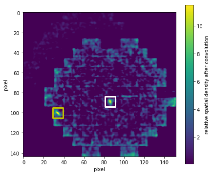
10-sigma+ density peaks marked with boxes.
Two peaks more than 10-sigma away from the median have been found in field 169. What is their nature? We don’t yet know; let’s take a look.
1.2.3.5.4. Simple Image Access (SIA)
Data Lab comes with batteries included. Now that we know the locations of two significant spatial overdensities, we can use the built-in Simple Image Access (SIA) service to retrieve from the Science Data Archive images taken at these positions.
The list of images that cover our RA & Dec positions is potentially long. Here we will ask for the deepest stacked images available in SMASH, in three bands (g,r,i).
For convenience, we write a little download function that takes the RA & Dec of a peak, and automates the retrieval of the desired image cutouts from the archive (see, e.g., this Jupyter notebook for the code).
We will also create a false-color 3-band composite image.
Let us inspect the images at the peak marked with a yellow box:
bands = list('gri')
idx = 1
images = download_deepest_images(tbl['ra'][idx], tbl['dec'][idx], fov=0.1, bands=bands) # FOV in deg
images = [im-np.median(im) for im in images] # subtract median from all images for better scaling
images += [make_lupton_rgb(*images[::-1],stretch=30)] # add a 3-color composite image; make_lupton_rgb() expects images in red,green,blue order
plot_images(images,geo=(4,1),titles=bands+['False-color 3-band image'])

.. code-block:: text

The full image list contains 2604 entries
Band g: downloading deepest stacked image...
Band r: downloading deepest stacked image...
Band i: downloading deepest stacked image...
Downloaded 3 images.
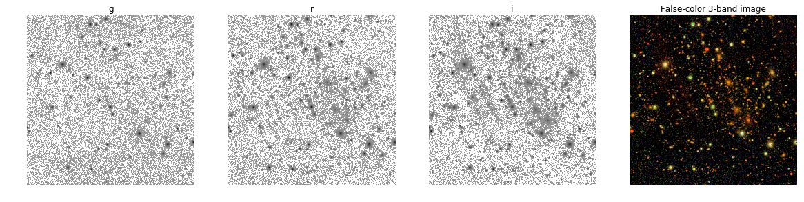
This seems to be a galaxy cluster. Interesting, but not the type of overdensity we are looking for.
Let’s do the same thing for the overdensity in the center of the field (marked with a white box).
idx = 0
images = download_deepest_images(tbl['ra'][idx], tbl['dec'][idx], fov=0.1, bands=bands) # FOV in deg
images = [im-np.median(im) for im in images] # subtract median from all images for better scaling
images += [make_lupton_rgb(*images[::-1],stretch=30)] # add a 3-color composite image
plot_images(images,titles=bands+['False-color 3-band image'])
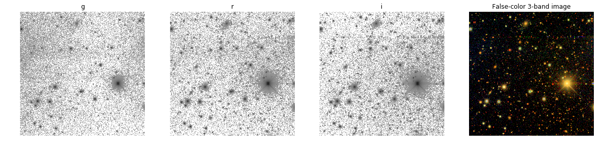
Defnitely not a galaxy cluster, just a faint stellar overdensity.
This is in fact the Hydra II dwarf galaxy, a Milky Way satellite.
1.2.3.5.5. Color-magnitude diagrams of the two overdensities
We can compare the color magnitude diagrams (CMD) of the two overdensities. We will query the SMASH catalog for all photometry within 5 arcminutes of the peak positions, but aren’t going to filter for blue stars this time.
def makequery(ra0,dec0,radius0=5./60.,field=169):
    query = """
      SELECT ra,dec,gmag,rmag,imag FROM smash_dr1.object
      WHERE fieldid = {:d}
        AND depthflag > 1
        AND abs(sharp) < 0.5
        AND gmag BETWEEN 9 AND 25
        AND q3c_radial_query(ra,dec,{:f},{:f},{:f})
      """.format(field,ra0,dec0,radius0)

    return query

 # the white box
 query0 = makequery(tbl['ra'][0],tbl['dec'][0]) # center ra & dec
 response = qc.query(sql=query0) # using sql argument instead of the default adql
 R0 = convert(response,'pandas')
 print(R0.head()) # a Pandas method
Returning Pandas dataframe
           ra        dec     gmag     rmag     imag
0  185.341390 -32.034610  18.7621  17.6098  17.1748
1  185.340696 -32.033947  24.6669      NaN      NaN
2  185.352840 -32.038977  24.8141  24.3438  23.9558
3  185.345295 -32.033874  24.7456  24.5389  24.4399
4  185.348514 -32.033831  24.8878  24.8343  24.7951
We can also compute colors:
R0['g_r'] = R0['gmag'] - R0['rmag']
print(R0.head())
           ra        dec     gmag     rmag     imag     g_r
0  185.341390 -32.034610  18.7621  17.6098  17.1748  1.1523
1  185.340696 -32.033947  24.6669      NaN      NaN     NaN
2  185.352840 -32.038977  24.8141  24.3438  23.9558  0.4703
3  185.345295 -32.033874  24.7456  24.5389  24.4399  0.2067
4  185.348514 -32.033831  24.8878  24.8343  24.7951  0.0535
After repeating for the yellow box, we plot the CMDs:
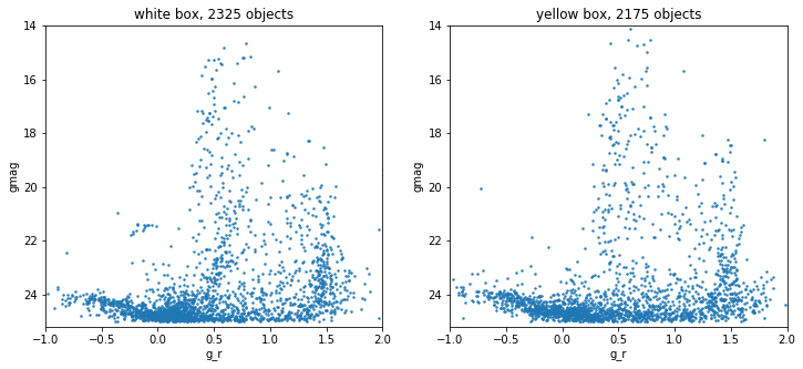
Color-magnitude diagrams.
Compare this to Vivas+2016 (5):
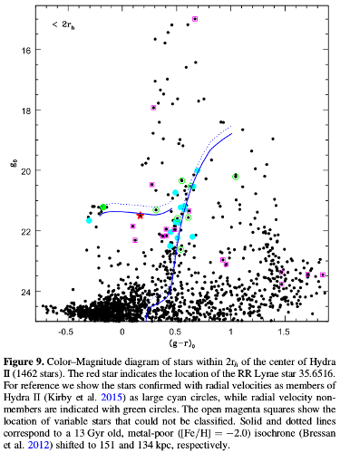
CMD of Hydra II from Vivas_2016
The blue solid line is the isochrone of a 13-Gyr old meta-poor population of stars, precisely what dominates faint MW dwarf galaxies. There’s also a hint of the Blue Horizontal Branch visible (at gmag ~ 21.8).
1.2.3.6. Output
If you wish, you can now save your photometry table for Hydra II to a local file and take it with you.
outfile = 'hydra2.csv'
R0.to_csv(outfile,index=False)
1.2.3.7. Links to resources
- 1
Martin et al. (2015, ApJ, 804, 5) “Hydra II: A Faint and Compact Milky Way Dwarf Galaxy Found in the Survey of the Magellanic Stellar History”: http://adsabs.harvard.edu/abs/2015ApJ…804L…5M
- 2(1,2)
Nidever, D. et al. (2017, AJ, 154, 199) “SMASH - Survey of the MAgellanic Stellar History”: http://adsabs.harvard.edu/abs/2017AJ….154..199N
- 3
Stanford et al. (2005, ApJ, 634, 2, L129) “An IR-selected Galaxy Cluster at z = 1.41”: http://adsabs.harvard.edu/abs/2005ApJ…634L.129S
- 4
Koposov et al. (2008, ApJ, 686, 279) “The Luminosity Function of the Milky Way Satellites”: http://adsabs.harvard.edu/abs/2008ApJ…686..279K
- 5
Vivas et al. 2016 (2016, AJ, 151, 118) “Variable Stars in the Field of the Hydra II Ultra-Faint Dwarf Galaxy”: http://adsabs.harvard.edu/abs/2016AJ….151..118V