Section author: Robert Nikutta <robert.nikutta@noirlab.edu>
1.2.4. Times series analysis of an RR Lyrae star in Hydra II
This document describes a science case that can be easily investigated with Data Lab.
The Jypter notebook file and a rendered HTML version are available on GitHub:
You will also find them on your Data Lab notebook server, in the notebooks-latest/
folder. [It’s best to first fetch the newest notebooks].
More on Jupyter notebooks.
Below we explain the motivation, methods, and Data Lab workflow, with snippets of the notebook in key places.
1.2.4.1. Background
One if the stars in the Hydra II dwarf galaxy is a variable RR Lyrae star. RR Lyrae pulsate due to the Kappa mechanism, with a period between a few hours and about one day. Due to their regular pulsations RR Lyrae stars can be used as standard candles for distance measurements.
1.2.4.2. Goal
The goal is to determine the period of the star’s light curve.
1.2.4.3. Data
The SMASH survey (1) provides all calibrated magnitudes and their
uncertainties, together with the time of observation, in the
source table of the smash_dr1 database in Data Lab. The
smash_dr1.source table also provides unique IDs for all objects in
the survey. We will retrieve the necessary data in the
Technique section below.
1.2.4.4. Technique
There are many period-finding algorithms used in literature, but most of them fall into one of two categories: Fourier-space based, and those trying to minimize phase dispersion when fitting a model to a lightcurve.
We will utilize one of the most popular algorithms from the Fourier-space based methods, the Lomb-Scargle periodogram (2, 3).
1.2.4.5. Data Lab Workflow
We will proceed with these steps:
retrieve the light curves (in several bands) of the RR Lyrae star from the SMASH database
compute the Lomb-Scargle periodogram of the light curve in one band (g band)
1.2.4.5.1. Data retrieval
We retrieve them e.g. with this query:
from dl import queryClient as qc

# Unique ID of a RR Lyrae star in Hydra II dwarf galaxy
objID = '169.429960'

# Select columns: RA, Dec, modified Julian date, calibrated mag, uncertainties, filter band
# Note: this database table encodes 'no measurement' values as 99.99
# Order the returned rows by ascending mod. Julian date
query = """SELECT ra,dec,mjd,cmag,cerr,filter
        FROM smash_dr1.source
        WHERE id='{:s}' AND cmag<99
        ORDER BY mjd ASC""".format(objID)
result = qc.query(query) # by default the result is a CSV formatted string
The selected columns are
modified Julian date (
mjd, in days)calibrated magnitudes (
cmag) and magnitude error (cerr)band filter name (
filter, as string)
We store them in a convenient Pandas dataframe:
from dl.helpers.utils import convert
df = convert(result,'pandas') # convert query result to a Pandas dataframe
print(df.head())
Returning Pandas dataframe
            mjd       cmag      cerr filter
0  56371.327538  21.433147  0.020651      g
1  56371.328563  21.231598  0.022473      r
2  56371.329582  21.149094  0.026192      i
3  56371.330610  21.237938  0.045429      z
4  56371.331633  21.346725  0.015112      g
1.2.4.5.2. Plot the lightcurve
With a little bit of matplotlib code we visualize the light curve in all bands (we define a small function for this in the notebook):
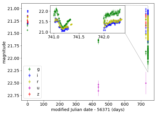
Lightcurve of the RR Lyrae star in Hydra II, in five bands. The inset shows a detailed view of the last 1.5 days worth of observations.
The last day of data is shown zoomed-in inside the plot inset.
1.2.4.5.3. Compute the Lomb-Scargle periodogram
Thanks to astropy, computing a Lomb-Scargle periodogram is a breeze. The code below is again wrapped in a little function inside the notebook:
# Select all measurements with the g band filter
sel = (df['filter'] == 'g')
t = df['mjd'][sel].values
y = df['cmag'][sel].values
dy = df['cerr'][sel].values

# Use astropy's LombScargle class
ls = stats.LombScargle(t, y)

# Compute the periodogram
#
# We guide the algorithm a bit:
#   min freq = 1/longest expected period (in days)
#   max freq = 1/shortest expected period (in days)
# RR Lyrae usually have a period of a fraction of one day
frequency, power = ls.autopower(minimum_frequency=1./1.,maximum_frequency=1./0.1)

period = 1./frequency # period is the inverse of frequency
best_period = 1./frequency[np.argmax(power)]  # period with most power / strongest signal

print("Best period: {:.3f} (days)".format(best_period))
Best period: 0.648 (days)
We find a best period of 0.648 days. Interestingly, 4 found 0.645 days using a complementary method (phase dispersion minimization). Excellent agreement.
The period is just the inverse of frequency. The best period or best frequency are those where the periodogram contains most power. Here the Lomb-Scargle periodogram:
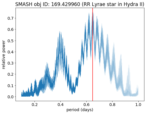
Lomb-Scargle periodogram.
1.2.4.5.4. Phase the lightcurve
With the best_period known, we can now “phase” the entire lightcurve (all 2+ years of it) with the best period, and compute the phase remainder of every date (x-axis data point). We then plot the “phased light curve”.
# light curve over period, take the remainder (i.e. the "phase" of one period)
phase = (t / best_period) % 1
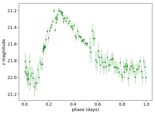
Phased light curve.
1.2.4.5.5. Compute and plot a simple Lomb-Scargle model
The LombScargle class can also compute a simple Lomb-Scargle model
for the observed light curve:
# compute t and y values
t_fit = np.linspace(phase.min(), phase.max())
y_fit = stats.LombScargle(t, y).model(t_fit, 1./best_period) # model() method expects time and best frequency
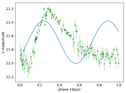
Simple Lomb-Scargle model fitted to the light curve.
Evidently this simple (sinusoidal) model is not an ideal model for the asymmetric RR Lyrae lightcurves. A better attempt would be to use either more physical models or template-based fitting (see e.g. 5).
1.2.4.5.6. Package your analysis into reusable code
All the plotting and analysis functions we defnined should of course
be put into a reusable Python module. We define a do_everything()
function that wraps all helper functions, and put the code into a
timeseries.py Python file. Then, repeating the analysis is just a
breeze:
import timeseries
timeseries.do_everything(df['ra'].values,df['dec'].values,t,y,dy)
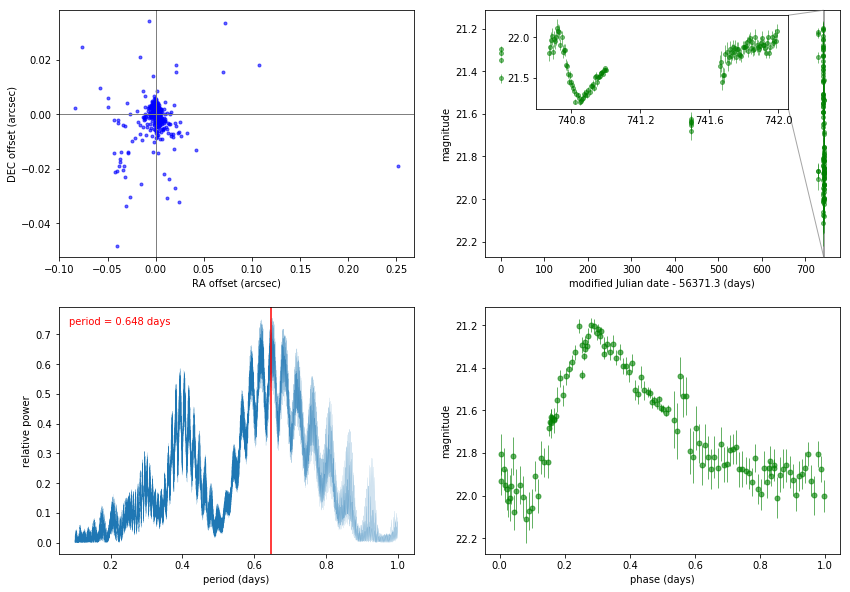
Repeatable and fast time series analysis.
1.2.4.6. Resources
- 1
Nidever, D. et al. (submitted) “SMASH - Survey of the MAgellanic Stellar History”, http://adsabs.harvard.edu/abs/2017arXiv170100502N
- 2
Lomb, N.R. (1976) “Least-squares frequency analysis of unequally spaced data”. Astrophysics and Space Science. 39 (2): 447–462, http://adsabs.harvard.edu/abs/1976Ap%26SS..39..447L
- 3
Scargle, J. D. (1982) “Studies in astronomical time series analysis. II - Statistical aspects of spectral analysis of unevenly spaced data”. Astrophysical Journal. 263: 835, http://adsabs.harvard.edu/doi/10.1086/160554
- 4
Vivas et al. 2016 (2016, AJ, 151, 118) “Variable Stars in the Field of the Hydra II Ultra-Faint Dwarf Galaxy”: http://adsabs.harvard.edu/abs/2016AJ….151..118V
- 5
Jake VanderPlas’ blog on Lomb-Scargle periodograms and on fitting RR Lyrae lightcurves with templates, https://jakevdp.github.io/blog/2015/06/13/lomb-scargle-in-python/